Top Qs
Timeline
Chat
Perspective
Dantzig–Wolfe decomposition
Algorithm for solving linear programming problems with special structure From Wikipedia, the free encyclopedia
Remove ads
Dantzig–Wolfe decomposition is an algorithm for solving (mixed integer) linear programming problems by exploiting their structure. It was originally developed by George Dantzig and Philip Wolfe and initially published in 1960.[1] Many texts on linear programming have sections dedicated to discussing this decomposition algorithm.[2][3][4][5][6][7] Dantzig–Wolfe decomposition can be used to improve the tractability of large-scale linear programs or create a tighter linear relaxation of mixed integer linear programs.
Remove ads
Explanation using column generation
Summarize
Perspective
The Dantzig-Wolfe decomposition considers the following initial linear program.
The decomposition starts by reformulating the problem. the constraint is equivalently reformulating by writing as a convex combination of points satisfying . This leads to the following linear program.
or equivalently
Here the new variables represent the coefficient in the convex combination, and the coefficients represent the points satisfying . In order to be exact, the formulation needs to contain one variable for each extreme point of the polyhedron induced by . This is because every point of a non-empty, bounded convex polyhedron can be represented as a convex combination of its extreme points. This leads to an intractable number of variables.
In order to be able to solve this new formulation containing an intractable number of variables, one use the column generation algorithm. This leads to an iterative algorithm where a couple is generated at every iteration.
Remarque: if the initial problem contains several constraints , , ... each of these constraints can be independently reformulated with the Dantzig-Wolfe method. This leads to independent sub-problems in the column generation algorithm. This fact is especially useful when the matrix constraint of the initial problem has a form of block diagonal structure.
The whole algorithm can be summarized as follows.
- Initialize the reformulated problem (P) with a small subset of the points and their corresponding variables ;
- Find an optimal solution of (P);
- Search for a point satisfying whose addition to (P) may improve the value of the optimal solution ;
- If such a point exists, add it to (P) and go to Step 2;
- Otherwise is optimal : stop.
It can be visualized as follows.
Remove ads
Exploiting special structure
Summarize
Perspective
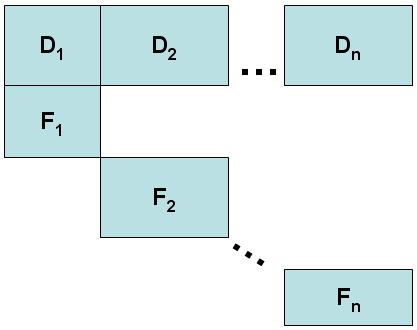
The main use case for the Dantzig–Wolfe decomposition is when the constraint matrix of the linear program has the following 'almost diagonal' structure visualized below.
Here, the set of constraints D is usually be identified as "connecting", "coupling", or "complicating" constraints. Meanwhile each constraint block is going to be reformulated using the Dantig-Wolfe method. This leads to one sub-problem for each block .
The two main reasons why the Dantzig-Wolfe method works especially well in this case are the following. First, each block only applies to a subset of the variables. This means the corresponding sub-problem will be a lot smaller than the original problem (less constraints and less variables) which means it can be solved faster. Second, although the sub-problem can always be solved independently, in the case of a diagonal structure the sub-problems are usually less linked. Indeed, suppose that and share a variable , then they have to 'agree' on the value of . This means every time the sub-problem proposes a new point with a different value for , the sub-problem also has to generate a new point with an agreeing value for . This slows down the overall process.
Remove ads
Implementation
Summarize
Perspective
There are examples of the implementation of Dantzig–Wolfe decomposition available in the closed source AMPL[8] and GAMS[9] mathematical modeling software. There are general, parallel, and fast implementations available as open-source software, including some provided by JuMP and the GNU Linear Programming Kit.[10]
The algorithm can be implemented such that the subproblems are solved in parallel, since their solutions are completely independent. When this is the case, there are options for the master program as to how the columns should be integrated into the master. The master may wait until each subproblem has completed and then incorporate all columns that improve the objective or it may choose a smaller subset of those columns. Another option is that the master may take only the first available column and then stop and restart all of the subproblems with new objectives based upon the incorporation of the newest column.
Another design choice for implementation involves columns that exit the basis at each iteration of the algorithm. Those columns may be retained, immediately discarded, or discarded via some policy after future iterations (for example, remove all non-basic columns every 10 iterations).
A (2001) computational evaluation of Dantzig-Wolfe in general and Dantzig-Wolfe and parallel computation is the PhD thesis by J. R. Tebboth[11]
See also
References
Wikiwand - on
Seamless Wikipedia browsing. On steroids.
Remove ads


