Discrete dipole approximation

The discrete dipole approximation (DDA), also known as the coupled dipole approximation, is a numerical method for computing the scattering and absorption of electromagnetic radiation by particles of arbitrary shape and composition. The method represents a continuum target as a finite array of small, polarizable dipoles, and solves for their interactions with the incident field and with each other. DDA can handle targets with inhomogeneous composition and anisotropic material properties, as well as periodic structures. It is widely applied in fields such as nanophotonics, radar scattering, aerosol physics, biomedical optics, and astrophysics.

Magnitude of the electric field strength ${\displaystyle E=|{\vec {E}}|}$ (colored) and the Poynting vector (black arrows) in the near field of the vertically oriented dipole in the image plane. Blue/red colors indicate an electric field oriented downwards/upwards.

Basic concepts

The basic idea of the DDA was introduced in 1964 by DeVoe^[1] who applied it to study the optical properties of molecular aggregates; retardation effects were not included, so DeVoe's treatment was limited to aggregates that were small compared with the wavelength. The DDA, including retardation effects, was proposed in 1973 by Purcell and Pennypacker^[2] who used it to study interstellar dust grains. Simply stated, the DDA is an approximation of the continuum target by a finite array of polarizable points. The points acquire dipole moments in response to the local electric field. The dipoles interact with one another via their electric fields, so the DDA is also sometimes referred to as the coupled dipole approximation.^[3][4]

Nature provides the physical inspiration for the DDA - in 1909 Lorentz^[5] showed that the dielectric properties of a substance could be directly related to the polarizabilities of the individual atoms of which it was composed, with a particularly simple and exact relationship, the Clausius-Mossotti relation (or Lorentz-Lorenz), when the atoms are located on a cubical lattice. We may expect that, just as a continuum representation of a solid is appropriate on length scales that are large compared with the interatomic spacing, an array of polarizable points can accurately approximate the response of a continuum target on length scales that are large compared with the interdipole separation.

For a finite array of point dipoles the scattering problem may be solved exactly, so the only approximation that is present in the DDA is the replacement of the continuum target by an array of N-point dipoles. The replacement requires specification of both the geometry (location of the dipoles) and the dipole polarizabilities. For monochromatic incident waves the self-consistent solution for the oscillating dipole moments may be found; from these the absorption and scattering cross sections are computed. If DDA solutions are obtained for two independent polarizations of the incident wave, then the complete amplitude scattering matrix can be determined. Alternatively, the DDA can be derived from volume integral equation for the electric field.^[6] This highlights that the approximation of point dipoles is equivalent to that of discretizing the integral equation, and thus decreases with decreasing dipole size.

With the recognition that the polarizabilities may be tensors, the DDA can readily be applied to anisotropic materials. The extension of the DDA to treat materials with nonzero magnetic susceptibility is also straightforward, although for most applications magnetic effects are negligible.

There are several reviews of DDA method. ^[7][6][8][9]

The method was improved by Draine, Flatau, and Goodman, who applied the fast Fourier transform to solve fast convolution problems arising in the discrete dipole approximation (DDA). This allowed for the calculation of scattering by large targets. They distributed an open-source code DDSCAT.^[7][10] There are now several DDA implementations,^[6] extensions to periodic targets,^[11] and particles placed on or near a plane substrate.^[12][13] Comparisons with exact techniques have also been published.^[14] Other aspects, such as the validity criteria of the discrete dipole approximation, were published.^[15] The DDA was also extended to employ rectangular or cuboid dipoles,^[16] which are more efficient for highly oblate or prolate particles.

Theory

In the discrete dipole approximation, a target object is represented as a finite array of N point dipoles located at positions ${\displaystyle \mathbf {r} _{j}}$ (${\displaystyle j=1,2,\dots ,N}$). The polarization vector ${\displaystyle \mathbf {P} _{j}}$ of each dipole is related to the local electric field ${\displaystyle \mathbf {E} _{j}}$ at that dipole by its polarizability tensor ${\displaystyle {\boldsymbol {\alpha }}_{j}}$:

In anisotropic case (diagonal polarizability)

${\displaystyle \mathbf {P} _{j}={\boldsymbol {\alpha }}_{j}\cdot \mathbf {E} _{j}}$

where ${\displaystyle {\boldsymbol {\alpha }}_{j}}$ is diagonal

${\displaystyle {\boldsymbol {\alpha }}_{j}={\begin{pmatrix}\alpha _{x,j}&0&0\\0&\alpha _{y,j}&0\\0&0&\alpha _{z,j}\end{pmatrix}}.}$

This leads to componentwise relations:

${\displaystyle {\begin{aligned}P_{x,j}&=\alpha _{x,j}E_{x,j},\\P_{y,j}&=\alpha _{y,j}E_{y,j},\\P_{z,j}&=\alpha _{z,j}E_{z,j}.\end{aligned}}}$

For isotropic materials, ${\displaystyle \alpha _{x,j}=\alpha _{y,j}=\alpha _{z,j}=\alpha _{j}}$, so

${\displaystyle \mathbf {P} _{j}=\alpha _{j}\mathbf {E} _{j}}$.

The local electric field ${\displaystyle \mathbf {E} _{j}}$ acting on the j‑th dipole is given by the sum of the incident field ${\displaystyle \mathbf {E} _{\mathrm {inc} }(\mathbf {r} _{j})}$ and the fields radiated by all other dipoles:

${\displaystyle \mathbf {E} _{j}=\mathbf {E} _{\mathrm {inc} }(\mathbf {r} _{j})+\sum _{k\neq j}\mathbf {G} (\mathbf {r} _{j}-\mathbf {r} _{k})\cdot \mathbf {P} _{k}}$

Here, ${\displaystyle \mathbf {G} (\mathbf {r} )}$ is the dyadic Green's function describing the field at position ${\displaystyle \mathbf {r} }$ due to a unit dipole at the origin.

Dyadic Green’s function

In the discrete dipole approximation, the electric field at dipole ${\displaystyle j}$ due to dipole ${\displaystyle k}$ is given by

${\displaystyle \mathbf {G} _{jk}={\frac {e^{ikr_{jk}}}{r_{jk}^{3}}}\left[k^{2}r_{jk}^{2}\left(\mathbf {I} -{\hat {\mathbf {r} }}_{jk}{\hat {\mathbf {r} }}_{jk}\right)+\left(1-ikr_{jk}\right)\left(3{\hat {\mathbf {r} }}_{jk}{\hat {\mathbf {r} }}_{jk}-\mathbf {I} \right)\right],}$

where ${\displaystyle \mathbf {r} _{jk}=\mathbf {r} _{j}-\mathbf {r} _{k}}$, ${\displaystyle r_{jk}=|\mathbf {r} _{jk}|}$, and ${\displaystyle {\hat {\mathbf {r} }}_{jk}=\mathbf {r} _{jk}/r_{jk}}$. Here ${\displaystyle \mathbf {I} }$ is the identity matrix and ${\displaystyle k=2\pi /\lambda }$ is the vacuum wavenumber.

Define

${\displaystyle C_{1}(r_{jk})={\frac {e^{ikr_{jk}}}{r_{jk}^{3}}}\left(k^{2}r_{jk}^{2}+ikr_{jk}-1\right),}$

${\displaystyle C_{2}(r_{jk})={\frac {e^{ikr_{jk}}}{r_{jk}^{3}}}\left(3-3ikr_{jk}-k^{2}r_{jk}^{2}\right).}$

The dyadic Green’s function ${\displaystyle \mathbf {G} _{jk}}$ is:

${\displaystyle \mathbf {G} _{jk}={\begin{pmatrix}C_{1}+C_{2}{\hat {r}}_{jk,x}^{2}&C_{2}{\hat {r}}_{jk,x}{\hat {r}}_{jk,y}&C_{2}{\hat {r}}_{jk,x}{\hat {r}}_{jk,z}\\C_{2}{\hat {r}}_{jk,y}{\hat {r}}_{jk,x}&C_{1}+C_{2}{\hat {r}}_{jk,y}^{2}&C_{2}{\hat {r}}_{jk,y}{\hat {r}}_{jk,z}\\C_{2}{\hat {r}}_{jk,z}{\hat {r}}_{jk,x}&C_{2}{\hat {r}}_{jk,z}{\hat {r}}_{jk,y}&C_{1}+C_{2}{\hat {r}}_{jk,z}^{2}\end{pmatrix}},}$

Notice that it is symmetric: ${\displaystyle G_{jk}^{yx}=G_{jk}^{xy},\;G_{jk}^{zx}=G_{jk}^{xz},\;G_{jk}^{zy}=G_{jk}^{yz}}$.

Here ${\displaystyle \mathbf {r} _{jk}=\mathbf {r} _{j}-\mathbf {r} _{k}}$ is the displacement vector from dipole ${\displaystyle k}$ to dipole ${\displaystyle j}$, ${\displaystyle r_{jk}=|\mathbf {r} _{jk}|}$ is the distance between them, and ${\displaystyle {\hat {\mathbf {r} }}_{jk}=\mathbf {r} _{jk}/r_{jk}}$ is the unit vector pointing from ${\displaystyle k}$ to ${\displaystyle j}$. The components of ${\displaystyle {\hat {\mathbf {r} }}_{jk}}$ are defined as:

${\displaystyle {\hat {r}}_{jk,x}={\frac {r_{j,x}-r_{k,x}}{r_{jk}}},\;{\hat {r}}_{jk,y}={\frac {r_{j,y}-r_{k,y}}{r_{jk}}},\;{\hat {r}}_{jk,z}={\frac {r_{j,z}-r_{k,z}}{r_{jk}}}.}$

Polarizability

Main article: Polarizability

In the discrete dipole approximation, the electromagnetic response of a target is modeled by replacing the continuous material with a finite array of point dipoles. Each dipole represents a small volume of the material and acts as a polarizable unit that interacts with both the incident field and the fields radiated by all other dipoles. The key parameter that describes how each dipole responds to the local electric field is its polarizability ${\displaystyle \alpha _{j}}$. For a homogeneous material, the polarizability of a dipole is determined by the material’s complex dielectric function ${\displaystyle \varepsilon (\lambda )}$, which depends on the wavelength ${\displaystyle \lambda }$ of light in vacuum. The dielectric function is related to the complex refractive index ${\displaystyle n=n'+in''}$ through ${\displaystyle \varepsilon =n^{2}}$. The goal in DDA is to assign to each dipole a polarizability ${\displaystyle \alpha _{j}}$ such that the array of dipoles reproduces, as accurately as possible, the scattering and absorption behavior of the original continuous medium. For isotropic materials, a common starting point is the Clausius–Mossotti relation, which connects the polarizability to the dielectric function:

In the discrete dipole approximation, the total volume of the target is divided into small cubic cells of volume ${\displaystyle V_{\mathrm {dipole} }=d^{3}}$, where ${\displaystyle d}$ is the lattice spacing. The Clausius–Mossotti polarizability for each dipole is

${\displaystyle \alpha _{j}={\frac {3V_{\mathrm {dipole} }}{4\pi }}{\frac {\varepsilon _{j}-1}{\varepsilon _{j}+2}},}$

where ${\displaystyle \varepsilon _{j}}$ is the relative permittivity of the material at the dipole’s position. The dipole volume ${\displaystyle V_{\mathrm {dipole} }}$ is constant across all dipoles.

This formula assumes that each dipole occupies a volume embedded in an otherwise uniform dielectric medium. In most implementations of DDA the formulation is expressed in Gaussian units (CGS). In these units, the polarizability ${\displaystyle \alpha _{j}}$ has dimensions of volume (cm³). In the discrete dipole approximation, the total volume of the target is divided into ${\displaystyle N}$ small cubic cells of volume ${\displaystyle V_{\mathrm {dipole} }=d^{3}}$, where ${\displaystyle d}$ is the lattice spacing and ${\displaystyle N}$ is the total number of dipoles. The total target volume is thus

${\displaystyle V_{\mathrm {target} }=Nd^{3}.}$

To improve the accuracy of the method various corrections to ${\displaystyle \alpha _{j}}$ are applied. These include: the lattice dispersion relation (LDR) polarizability (Draine & Goodman, 1993), which adjusts ${\displaystyle \alpha _{j}}$ to ensure that the dispersion relation of an infinite lattice of dipoles matches that of the continuous material; the radiative reaction (RR) correction, which compensates for the fact that each dipole radiates energy and is influenced by its own radiation field.

Size parameter

The size parameter is a dimensionless quantity used in scattering theory to characterize the size of a particle relative to the wavelength of the incident light. For a sphere, it is defined as:

${\displaystyle x={\frac {2\pi r}{\lambda }}=kr}$

where: ${\displaystyle x}$ is the size parameter (dimensionless), ${\displaystyle a}$ is the radius of the sphere, ${\displaystyle \lambda }$ is the wavelength of light in vacuum,

${\displaystyle k={\frac {2\pi }{\lambda }}}$ is the wavenumber.

In case of a sphere, the size parameter determines the scattering regime:

• If ${\displaystyle x\ll 1}$, [Rayleigh scattering|Rayleigh scattering]] dominates.
• If ${\displaystyle x\sim 1}$, the scattering is in the regime of Mie scattering.
• If ${\displaystyle x\gg 1}$, the geometric optics approximation becomes valid.

Effective radius and dipole discretization

For nonspherical targets with the same volume as a sphere, the effective radius ${\displaystyle r_{\text{eff}}}$ is often used in place of ${\displaystyle r}$, with:

${\displaystyle r_{\text{eff}}=\left({\frac {3V_{\text{tot}}}{4\pi }}\right)^{1/3}=\left({\frac {3Nd^{3}}{4\pi }}\right)^{1/3}}$

where: ${\displaystyle N}$ is the total number of dipoles, ${\displaystyle d}$ is the dipole spacing, ${\displaystyle V_{\text{tot}}=Nd^{3}}$ is the total volume represented by the dipoles. This gives effective size parameter

${\displaystyle x_{\text{eff}}={\frac {2\pi r_{\text{eff}}}{\lambda }}}$

One convenient trick in certain DDA accuracy tests is to define wavelength as ${\displaystyle 2\pi }$, in such a case effective radius is the same as effective size parameter.

Dipole-scale size parameter

Each polarizable point (dipole) occupies a cubic volume with side length ${\displaystyle d}$. Analogous to the global size parameter ${\displaystyle x=2\pi r/\lambda }$ used for whole particles, one can define a local size parameter for each dipole:

${\displaystyle x_{d}=|m|kd={\frac {2\pi |m|d}{\lambda }}}$

This local parameter quantifies the ratio of the dipole size to the wavelength of light inside the material. For the DDA to be accurate, the field should vary slowly over the size of each dipole. This condition is satisfied when:

${\displaystyle x_{d}=|m|kd\lesssim 0.5}$

This ensures that each dipole is optically small, fields vary slowly over the dipole and the polarizability formula used for each dipole is accurate. Notice that a similar parameter plays a crucial role in the anomalous diffraction theory of van de Hulst, where the total phase shift experienced by light rays traveling through or around the particle is given by:

${\displaystyle \delta =2\pi (m-1){\frac {r}{\lambda }}}$

This describes the optical path difference introduced by the particle (or in the case of DDA by a dipole).

Explicit Matrix Form of the DDA System

The Discrete Dipole Approximation (DDA) linear system is expressed as:

${\displaystyle \mathbf {A} \mathbf {P} =\mathbf {E} _{\mathrm {inc} }}$

Let N be the number of dipoles. Each dipole has a polarization vector ${\displaystyle \mathbf {P} _{j}\in \mathbb {C} ^{3}}$. The total system is a matrix equation of size ${\displaystyle 3N\times 3N}$:

${\displaystyle {\begin{bmatrix}{\boldsymbol {\alpha }}_{1}^{-1}&-\mathbf {G} _{12}&-\mathbf {G} _{13}&\cdots &-\mathbf {G} _{1N}\\-\mathbf {G} _{21}&{\boldsymbol {\alpha }}_{2}^{-1}&-\mathbf {G} _{23}&\cdots &-\mathbf {G} _{2N}\\-\mathbf {G} _{31}&-\mathbf {G} _{32}&{\boldsymbol {\alpha }}_{3}^{-1}&\cdots &-\mathbf {G} _{3N}\\\vdots &\vdots &\vdots &\ddots &\vdots \\-\mathbf {G} _{N1}&-\mathbf {G} _{N2}&-\mathbf {G} _{N3}&\cdots &{\boldsymbol {\alpha }}_{N}^{-1}\end{bmatrix}}{\begin{bmatrix}\mathbf {P} _{1}\\\mathbf {P} _{2}\\\vdots \\\mathbf {P} _{N}\end{bmatrix}}={\begin{bmatrix}\mathbf {E} _{\mathrm {inc} ,1}\\\mathbf {E} _{\mathrm {inc} ,2}\\\vdots \\\mathbf {E} _{\mathrm {inc} ,N}\end{bmatrix}}}$

Each block ${\displaystyle \mathbf {A} _{jk}}$ is a ${\displaystyle 3\times 3}$ complex matrix, defined by:

${\displaystyle \mathbf {A} _{jk}={\begin{cases}{\boldsymbol {\alpha }}_{j}^{-1},&{\text{if }}j=k\\-\mathbf {G} _{jk},&{\text{if }}j\neq k\end{cases}}}$

where: ${\displaystyle {\boldsymbol {\alpha }}_{j}^{-1}\in \mathbb {C} ^{3\times 3}}$ is the inverse polarizability tensor, ${\displaystyle \mathbf {G} _{jk}\in \mathbb {C} ^{3\times 3}}$ is the dyadic Green’s tensor for interaction between dipoles ${\displaystyle j}$ and ${\displaystyle k}$, ${\displaystyle \mathbf {P} _{j},\mathbf {E} _{\mathrm {inc} ,j}\in \mathbb {C} ^{3}}$ are the dipole polarization and incident electric field at dipole ${\displaystyle j}$, respectively.

Typically dipoles are arranged on a regular grid. This implies translational invariance:

${\displaystyle \mathbf {G} _{jk}=\mathbf {G} (\mathbf {r} _{j}-\mathbf {r} _{k})=\mathbf {G} _{|j-k|}}$

Because ${\displaystyle \mathbf {G} _{|j-k|}=\mathbf {G} _{|k-j|}}$, the matrix ${\displaystyle \mathbf {A} }$ is symmetric:

${\displaystyle \mathbf {A} _{jk}=\mathbf {A} _{kj}\quad {\text{for all }}j,k}$

As a result, the interaction matrix ${\displaystyle \mathbf {A} }$ is a block Toeplitz symmetric matrix.

Fast Fourier Transform for fast convolution calculations

The Fast Fourier Transform (FFT) method was introduced in 1991 by Goodman, Draine, and Flatau^[17] for the discrete dipole approximation. They utilized a 3D FFT GPFA written by Clive Temperton. The interaction matrix was extended to twice its original size to incorporate negative lags by mirroring and reversing the interaction matrix. Several variants have been developed since then. Barrowes, Teixeira, and Kong^[18] in 2001 developed a code that uses block reordering, zero padding, and a reconstruction algorithm, claiming minimal memory usage. McDonald, Golden, and Jennings^[19] in 2009 used a 1D FFT code and extended the interaction matrix in the x, y, and z directions of the FFT calculations, suggesting memory savings due to this approach. This variant was also implemented in the MATLAB 2021 code by Shabaninezhad and Ramakrishna^[20]. Other techniques to accelerate convolutions have been suggested in a general context^[21][22] along with faster evaluations of Fast Fourier Transforms arising in DDA problem solvers.

Conjugate gradient iteration schemes and preconditioning

Some of the early calculations of the polarization vector were based on direct inversion^[2] and the implementation of the conjugate gradient method by Petravic and Kuo-Petravic.^[23] Subsequently, many other conjugate gradient methods have been tested.^[24] Advances in the preconditioning of linear systems of equations arising in the DDA setup have also been reported.^[25]

Thermal discrete dipole approximation

Thermal discrete dipole approximation is an extension of the original DDA to simulations of near-field heat transfer between 3D arbitrarily-shaped objects.^[26][27]

Discrete dipole approximation codes

Main article: Discrete dipole approximation codes

Most of the codes apply to arbitrary-shaped inhomogeneous nonmagnetic particles and particle systems in free space or homogeneous dielectric host medium. The calculated quantities typically include the Mueller matrices, integral cross-sections (extinction, absorption, and scattering), internal fields and angle-resolved scattered fields (phase function). There are some published comparisons of existing DDA codes.^[14]

Gallery of shapes

• 
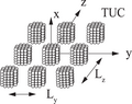  Scattering by periodic structures such as slabs, gratings, of periodic cubes placed on a surface, can be solved in the discrete dipole approximation.
• 
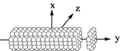  Scattering by infinite object (such as cylinder) can be solved in the discrete dipole approximation.

See also

• Computational electromagnetics
• Mie theory
• Finite-difference time-domain method
• Method of moments (electromagnetics)