Lorenz system

Not to be confused with Lorenz curve or Lorentz distribution.

The Lorenz system is a set of three ordinary differential equations, first developed by the meteorologist Edward Lorenz while studying atmospheric convection. It is a classic example of a system that can exhibit chaotic behavior, meaning its output can be highly sensitive to small changes in its starting conditions.

A sample solution in the Lorenz attractor when ρ = 28, σ = 10, and β = ⁠8/3⁠

For certain values of its parameters, the system's solutions form a complex, looping pattern known as the Lorenz attractor. The shape of this attractor, when graphed, is famously said to resemble a butterfly. The system's extreme sensitivity to initial conditions gave rise to the popular concept of the butterfly effect—the idea that a small event, like the flap of a butterfly's wings, could ultimately alter large-scale weather patterns. While the system is deterministic—its future behavior is fully determined by its initial conditions—its chaotic nature makes long-term prediction practically impossible.

Overview

See also: Chaos theory § Lorenz's pioneering contributions to chaotic modeling

In 1963, Edward Lorenz developed the system as a simplified mathematical model for atmospheric convection.^[1] He was attempting to model the way air moves when heated from below and cooled from above. The model describes how three key properties of this system change over time:

• x is proportional to the intensity of the convection (the rate of fluid flow).
• y is proportional to the temperature difference between the rising and falling air currents.
• z is proportional to the distortion of the vertical temperature profile from a linear one.

The model was developed with the assistance of Ellen Fetter, who performed the numerical simulations and created the figures,^[1] and Margaret Hamilton, who aided in the initial computations.^[2] The behavior of these three variables is governed by the following equations:

${\displaystyle {\begin{aligned}{\frac {\mathrm {d} x}{\mathrm {d} t}}&=\sigma (y-x),\\[6pt]{\frac {\mathrm {d} y}{\mathrm {d} t}}&=x(\rho -z)-y,\\[6pt]{\frac {\mathrm {d} z}{\mathrm {d} t}}&=xy-\beta z.\end{aligned}}}$

The constants σ, ρ, and β are parameters representing physical properties of the system: σ is the Prandtl number, ρ is the Rayleigh number, and β relates to the physical dimensions of the fluid layer itself.^[3]

From a technical standpoint, the Lorenz system is nonlinear, aperiodic, three-dimensional, and deterministic. While originally for weather, the equations have since been found to model behavior in a wide variety of systems, including lasers,^[4] dynamos,^[5] electric circuits,^[6] and even some chemical reactions.^[7] The Lorenz equations have been the subject of hundreds of research articles and at least one book-length study.^[3]

Analysis

One normally assumes that the parameters σ, ρ, and β are positive. Lorenz used the values σ = 10, ρ = 28, and β = ⁠8/3⁠. The system exhibits chaotic behavior for these (and nearby) values.^[8]

If ρ < 1 then there is only one equilibrium point, which is at the origin. This point corresponds to no convection. All orbits converge to the origin, which is a global attractor, when ρ < 1.^[9]

A pitchfork bifurcation occurs at ρ = 1, and for ρ > 1 two additional critical points appear at$${\displaystyle \left({\sqrt {\beta (\rho -1)}},{\sqrt {\beta (\rho -1)}},\rho -1\right)\quad {\text{and}}\quad \left(-{\sqrt {\beta (\rho -1)}},-{\sqrt {\beta (\rho -1)}},\rho -1\right).}$$ These correspond to steady convection. This pair of equilibrium points is stable only if

${\displaystyle \rho <\sigma {\frac {\sigma +\beta +3}{\sigma -\beta -1}},}$

which can hold only for positive ρ if σ > β + 1. At the critical value, both equilibrium points lose stability through a subcritical Hopf bifurcation.^[10]

When ρ = 28, σ = 10, and β = ⁠8/3⁠, the Lorenz system has chaotic solutions (but not all solutions are chaotic). Almost all initial points will tend to an invariant set – the Lorenz attractor – a strange attractor, a fractal, and a self-excited attractor with respect to all three equilibria. Its Hausdorff dimension is estimated from above by the Lyapunov dimension (Kaplan-Yorke dimension) as 2.06±0.01,^[11] and the correlation dimension is estimated to be 2.05±0.01.^[12] The exact Lyapunov dimension formula of the global attractor can be found analytically under classical restrictions on the parameters:^[13][11][14]

${\displaystyle 3-{\frac {2(\sigma +\beta +1)}{\sigma +1+{\sqrt {\left(\sigma -1\right)^{2}+4\sigma \rho }}}}}$

The Lorenz attractor is difficult to analyze, but the action of the differential equation on the attractor is described by a fairly simple geometric model.^[15] Proving that this is indeed the case is the fourteenth problem on the list of Smale's problems. This problem was the first one to be resolved, by Warwick Tucker in 2002.^[16]

For other values of ρ, the system displays knotted periodic orbits. For example, with ρ = 99.96 it becomes a T(3,2) torus knot.

Example solutions of the Lorenz system for different values of ρ
ρ = 14, σ = 10, β = ⁠8/3⁠ (Enlarge)	ρ = 13, σ = 10, β = ⁠8/3⁠ (Enlarge)
ρ = 15, σ = 10, β = ⁠8/3⁠ (Enlarge)	ρ = 28, σ = 10, β = ⁠8/3⁠ (Enlarge)
For small values of ρ, the system is stable and evolves to one of two fixed point attractors. When ρ > 24.74, the fixed points become repulsors and the trajectory is repelled by them in a very complex way.

Sensitive dependence on the initial condition
Time t = 1 (Enlarge)	Time t = 2 (Enlarge)	Time t = 3 (Enlarge)
These figures — made using ρ = 28, σ = 10, and β = ⁠8/3⁠ — show three time segments of the 3-D evolution of two trajectories (one in blue, the other in yellow) in the Lorenz attractor starting at two initial points that differ only by 10−5 in the x-coordinate. Initially, the two trajectories seem coincident (only the yellow one can be seen, as it is drawn over the blue one) but, after some time, the divergence is obvious.

Divergence of nearby trajectories.
Evolution of three initially nearby trajectories of the Lorenz system. In this animation the equation is numerically integrated using a Runge-Kutta routine — made using starting from three initial conditions (0.9,0,0) (green), (1.0,0,0) (blue) and (1.1,0,0) (red). Produced with WxMaxima.
The parameters are: ${\displaystyle \rho =28}$, ${\displaystyle \sigma =10}$, and ${\displaystyle \beta =8/3}$ . Significant divergence is seen at around ${\displaystyle t=24.0}$, beyond which the trajectories become uncorrelated. The full-sized graphic can be accessed here.

Connection to tent map

A recreation of Lorenz's results created on Mathematica. Points above the red line correspond to the system switching lobes.

In Figure 4 of his paper,^[1] Lorenz plotted the relative maximum value in the z direction achieved by the system against the previous relative maximum in the z direction. This procedure later became known as a Lorenz map (not to be confused with a Poincaré plot, which plots the intersections of a trajectory with a prescribed surface). The resulting plot has a shape very similar to the tent map. Lorenz also found that when the maximum z value is above a certain cut-off, the system will switch to the next lobe. Combining this with the chaos known to be exhibited by the tent map, he showed that the system switches between the two lobes chaotically.

A Generalized Lorenz System

Over the past several years, a series of papers regarding high-dimensional Lorenz models have yielded a generalized Lorenz model,^[17] which can be simplified into the classical Lorenz model for three state variables or the following five-dimensional Lorenz model for five state variables:^[18]$${\displaystyle {\begin{aligned}{\frac {\mathrm {d} x}{\mathrm {d} t}}&=\sigma (y-x),\\[6pt]{\frac {\mathrm {d} y}{\mathrm {d} t}}&=x(\rho -z)-y,\\[6pt]{\frac {\mathrm {d} z}{\mathrm {d} t}}&=xy-xy_{1}-\beta z,\\[6pt]{\frac {\mathrm {d} y_{1}}{\mathrm {d} t}}&=xz-2xz_{1}-d_{0}y_{1},\\[6pt]{\frac {\mathrm {d} z_{1}}{\mathrm {d} t}}&=2xy_{1}-4\beta z_{1}.\end{aligned}}}$$

A choice of the parameter ${\textstyle d_{0}={\dfrac {19}{3}}}$ has been applied to be consistent with the choice of the other parameters. See details in.^[17][18]

Simulations

Julia Simulation

Julia simulation

using Plots
# define the Lorenz attractor
@kwdef mutable struct Lorenz
    dt::Float64 = 0.02
    σ::Float64 = 10
    ρ::Float64 = 28
    β::Float64 = 8/3
    x::Float64 = 2
    y::Float64 = 1
    z::Float64 = 1
end

function step!(l::Lorenz)
    dx = l.σ * (l.y - l.x)
    dy = l.x * (l.ρ - l.z) - l.y
    dz = l.x * l.y - l.β * l.z
    l.x += l.dt * dx
    l.y += l.dt * dy
    l.z += l.dt * dz
end

attractor = Lorenz()

# initialize a 3D plot with 1 empty series
plt = plot3d(
    1,
    xlim = (-30, 30),
    ylim = (-30, 30),
    zlim = (0, 60),
    title = "Lorenz Attractor",
    marker = 2,
)

# build an animated gif by pushing new points to the plot, saving every 10th frame
@gif for i=1:1500
    step!(attractor)
    push!(plt, attractor.x, attractor.y, attractor.z)
end every 10

Maple simulation

deq := [diff(x(t), t) = 10*(y(t) - x(t)), diff(y(t), t) = 28*x(t) - y(t) - x(t)*z(t), diff(z(t), t) = x(t)*y(t) - 8/3*z(t)]:
with(DEtools):
DEplot3d(deq, {x(t), y(t), z(t)}, t = 0 .. 100, [[x(0) = 10, y(0) = 10, z(0) = 10]], stepsize = 0.01, x = -20 .. 20, y = -25 .. 25, z = 0 .. 50, linecolour = sin(t*Pi/3), thickness = 1, orientation = [-40, 80], title = `Lorenz Chaotic Attractor`);

Maxima simulation

[sigma, rho, beta]: [10, 28, 8/3]$
eq: [sigma*(y-x), x*(rho-z)-y, x*y-beta*z]$
sol: rk(eq, [x, y, z], [1, 0, 0], [t, 0, 50, 1/100])$
len: length(sol)$
x: makelist(sol[k][2], k, len)$
y: makelist(sol[k][3], k, len)$
z: makelist(sol[k][4], k, len)$
draw3d(points_joined=true, point_type=-1, points(x, y, z), proportional_axes=xyz)$

MATLAB simulation

% Solve over time interval [0,100] with initial conditions [1,1,1]
% ''f'' is set of differential equations
% ''a'' is array containing x, y, and z variables
% ''t'' is time variable

sigma = 10;
beta = 8/3;
rho = 28;
f = @(t,a) [-sigma*a(1) + sigma*a(2); rho*a(1) - a(2) - a(1)*a(3); -beta*a(3) + a(1)*a(2)];
[t,a] = ode45(f,[0 100],[1 1 1]);     % Runge-Kutta 4th/5th order ODE solver
plot3(a(:,1),a(:,2),a(:,3))

Mathematica simulation

Standard way:

tend = 50;
eq = {x'[t] == σ (y[t] - x[t]), 
      y'[t] == x[t] (ρ - z[t]) - y[t], 
      z'[t] == x[t] y[t] - β z[t]};
init = {x[0] == 10, y[0] == 10, z[0] == 10};
pars = {σ->10, ρ->28, β->8/3};
{xs, ys, zs} = 
  NDSolveValue[{eq /. pars, init}, {x, y, z}, {t, 0, tend}];
ParametricPlot3D[{xs[t], ys[t], zs[t]}, {t, 0, tend}]

Less verbose:

lorenz = NonlinearStateSpaceModel[{{σ (y - x), x (ρ - z) - y, x y - β z}, {}}, {x, y, z}, {σ, ρ, β}];
soln[t_] = StateResponse[{lorenz, {10, 10, 10}}, {10, 28, 8/3}, {t, 0, 50}];
ParametricPlot3D[soln[t], {t, 0, 50}]

Python simulation

import matplotlib.pyplot as plt
import numpy as np

def lorenz(xyz, *, s=10, r=28, b=2.667):
    """
    Parameters
    ----------
    xyz : array-like, shape (3,)
       Point of interest in three-dimensional space.
    s, r, b : float
       Parameters defining the Lorenz attractor.

    Returns
    -------
    xyz_dot : array, shape (3,)
       Values of the Lorenz attractor's partial derivatives at *xyz*.
    """
    x, y, z = xyz
    x_dot = s*(y - x)
    y_dot = r*x - y - x*z
    z_dot = x*y - b*z
    return np.array([x_dot, y_dot, z_dot])

dt = 0.01
num_steps = 10000

xyzs = np.empty((num_steps + 1, 3))  # Need one more for the initial values
xyzs[0] = (0., 1., 1.05)  # Set initial values
# Step through "time", calculating the partial derivatives at the current point
# and using them to estimate the next point
for i in range(num_steps):
    xyzs[i + 1] = xyzs[i] + lorenz(xyzs[i]) * dt

# Plot
ax = plt.figure().add_subplot(projection='3d')

ax.plot(*xyzs.T, lw=0.6)
ax.set_xlabel("X Axis")
ax.set_ylabel("Y Axis")
ax.set_zlabel("Z Axis")
ax.set_title("Lorenz Attractor")

plt.show()

R Simulation

R simulation

library(deSolve)
library(plotly)
# parameters
prm <- list(sigma = 10, rho = 28, beta = 8/3)
# initial values
varini <- c(
  X = 1,
  Y = 1, 
  Z = 1
)

Lorenz <- function (t, vars, prm) {
  with(as.list(vars), {
    dX <- prm$sigma*(Y - X)
    dY <- X*(prm$rho - Z) - Y
    dZ <- X*Y - prm$beta*Z
    return(list(c(dX, dY, dZ)))
   })
}

times <- seq(from = 0, to = 100, by = 0.01)
# call ode solver
out <- ode(y = varini, times = times, func = Lorenz,
           parms = prm)

# to assign color to points
gfill <- function (repArr, long) {
  rep(repArr, ceiling(long/length(repArr)))[1:long]
}

dout <- as.data.frame(out)

dout$color <- gfill(rainbow(10), nrow(dout))

# Graphics production with Plotly:
plot_ly(
  data=dout, x = ~X, y = ~Y, z = ~Z,
  type = 'scatter3d', mode = 'lines',
  opacity = 1, line = list(width = 6, color = ~color, reverscale = FALSE)
)

plot the solutions of Lorenz ode system

plot every ${\displaystyle y_{1}}$, ${\displaystyle y_{2}}$, and ${\displaystyle y_{3}}$ in terms of ${\displaystyle t}$ time

plot the ${\displaystyle y}$ against ${\displaystyle x}$ or equivalently ${\displaystyle y_{2}}$ against ${\displaystyle y_{2}}$

plot the ${\displaystyle z}$ against ${\displaystyle x}$ or equivalently ${\displaystyle y_{3}}$ against ${\displaystyle y_{1}}$

plot the ${\displaystyle z}$ against ${\displaystyle y}$ or equivalently ${\displaystyle y_{3}}$ against ${\displaystyle y_{2}}$

SageMath simulation

We try to solve this system of equations for ${\displaystyle \rho =28}$, ${\displaystyle \sigma =10}$, ${\displaystyle \beta ={\frac {8}{3}}}$, with initial conditions ${\displaystyle y_{1}(0)=0}$, ${\displaystyle y_{2}(0)=0.5}$, ${\displaystyle y_{3}(0)=0}$.

# we solve the Lorenz system of the differential equations.
# Runge-Kutta's method y_{n+1}= y_n + h*(k_1 + 2*k_2+2*k_3+k_4)/6; x_{n+1}=x_n+h
# k_1=f(x_n,y_n), k_2=f(x_n+h/2, y_n+hk_1/2), k_3=f(x_n+h/2, y_n+hk_2/2), k_4=f(x_n+h, y_n+hk_3)
# differential equation
def Runge_Kutta(f,v,a,b,h,n):
    tlist = [a+i*h for i in range(n+1)]
    y = [[0,0,0] for _ in range(n+1)]
    # Taking length of f (number of equations).
    m=len(f)
    # Number of variables in v.
    vm=len(v)
    if m!=vm:
        return("error, number of equations is not equal with the number of variables.")
    for r in range(vm):
        y[0][r]=b[r]
    # making a vector and component will be a list    
    # main part of the algorithm    
    k1=[0 for _ in range(m)]
    k2=[0 for _ in range(m)]
    k3=[0 for _ in range(m)]
    k4=[0 for _ in range(m)]
    for i in range(1,n+1): # for each t_i, i=1, ... , n
        # k1=h*f(t_{i-1},x_1(t_{i-1}),...,x_m(t_{i-1}))
        for j in range(m): # for each f_{j+1}, j=0, ... , m-1
            k1[j]=f[j].subs(t==tlist[i-1])
            for r in range(vm):
                k1[j]=k1[j].subs(v[r]==y[i-1][r])
            k1[j]=h*k1[j]
        for j in range(m): # k2=h*f(t_{i-1}+h/2,x_1(t_{i-1})+k1/2,...,x_m(t_{i-1}+k1/2))
            k2[j]=f[j].subs(t==tlist[i-1]+h/2)
            for r in range(vm):
                k2[j]=k2[j].subs(v[r]==y[i-1][r]+k1[r]/2)
            k2[j]=h*k2[j]
        for j in range(m): # k3=h*f(t_{i-1}+h/2,x_1(t_{i-1})+k2/2,...,x_m(t_{i-1})+k2/2)
            k3[j]=f[j].subs(t==tlist[i-1]+h/2)
            for r in range(vm):
                k3[j]=k3[j].subs(v[r]==y[i-1][r]+k2[r]/2)
            k3[j]=h*k3[j]
        for j in range(m): # k4=h*f(t_{i-1}+h,x_1(t_{i-1})+k3,...,x_m(t_{i-1})+k3)
            k4[j]=f[j].subs(t==tlist[i-1]+h)
            for r in range(vm):
                k4[j]=k4[j].subs(v[r]==y[i-1][r]+k3[r])
            k4[j]=h*k4[j]
        for j in range(m): # Now x_j(t_i)=x_j(t_{i-1})+(k1+2k2+2k3+k4)/6
            y[i][j]=y[i-1][j]+(k1[j]+2*k2[j]+2*k3[j]+k4[j])/6
    return(tlist,y)

# (Figure 1) Here, we plot the solutions of the Lorenz ODE system. 
a=0.0 # t_0
b=[0.0,.50,0.0] # x_1(t_0), ... , x_m(t_0)
t=var('t')
x = var('x', n=3, latex_name='x')
v=[x[ii] for ii in range(3)]
f= [10*(x1-x0),x0*(28-x2)-x1,x0*x1-(8/3)*x2];
n=1600
h=0.0125
tlist,y=Runge_Kutta(f,v,a,b,h,n)
#print(tlist)
#print(y)
T=point3d([[y[i][0],y[i][1],y[i][2]] for i in range(n)], color='red')
S=line3d([[y[i][0],y[i][1],y[i][2]] for i in range(n)], color='red')
show(T+S)

# (Figure 2) Here, we plot every y1, y2, and y3 in terms of time.
a=0.0 # t_0
b=[0.0,.50,0.0] # x_1(t_0), ... , x_m(t_0)
t=var('t')
x = var('x', n=3, latex_name='x')
v=[x[ii] for ii in range(3)]
Lorenz= [10*(x1-x0),x0*(28-x2)-x1,x0*x1-(8/3)*x2];
n=100
h=0.1
tlist,y=Runge_Kutta(Lorenz,v,a,b,h,n)
#Runge_Kutta(f,v,0,b,h,n)
#print(tlist)
#print(y)
P1=list_plot([[tlist[i],y[i][0]] for i in range(n)], plotjoined=True, color='red');
P2=list_plot([[tlist[i],y[i][1]] for i in range(n)], plotjoined=True, color='green');
P3=list_plot([[tlist[i],y[i][2]] for i in range(n)], plotjoined=True, color='yellow');
show(P1+P2+P3)

# (Figure 3) Here, we plot the y and x or equivalently y2 and y1 
a=0.0 # t_0
b=[0.0,.50,0.0] # x_1(t_0), ... , x_m(t_0)
t=var('t')
x = var('x', n=3, latex_name='x')
v=[x[ii] for ii in range(3)]
f= [10*(x1-x0),x0*(28-x2)-x1,x0*x1-(8/3)*x2];
n=800
h=0.025
tlist,y=Runge_Kutta(f,v,a,b,h,n)
vv=[[y[i][0],y[i][1]] for i in range(n)];
#print(tlist)
#print(y)
T=points(vv, rgbcolor=(0.2,0.6, 0.1), pointsize=10)
S=line(vv,rgbcolor=(0.2,0.6, 0.1))
show(T+S)

# (Figure 4) Here, we plot the z and x or equivalently y3 and y1 
a=0.0 # t_0
b=[0.0,.50,0.0] # x_1(t_0), ... , x_m(t_0)
t=var('t')
x = var('x', n=3, latex_name='x')
v=[x[ii] for ii in range(3)]
f= [10*(x1-x0),x0*(28-x2)-x1,x0*x1-(8/3)*x2];
n=800
h=0.025
tlist,y=Runge_Kutta(f,v,a,b,h,n)
vv=[[y[i][0],y[i][2]] for i in range(n)];
#print(tlist)
#print(y)
T=points(vv, rgbcolor=(0.2,0.6, 0.1), pointsize=10)
S=line(vv,rgbcolor=(0.2,0.6, 0.1))
show(T+S)

# (Figure 5) Here, we plot the z and x or equivalently y3 and y2 
a=0.0 # t_0
b=[0.0,.50,0.0] # x_1(t_0), ... , x_m(t_0)
t=var('t')
x = var('x', n=3, latex_name='x')
v=[x[ii] for ii in range(3)]
f= [10*(x1-x0),x0*(28-x2)-x1,x0*x1-(8/3)*x2];
n=800
h=0.025
tlist,y=Runge_Kutta(f,v,a,b,h,n)
vv=[[y[i][1],y[i][2]] for i in range(n)];
#print(tlist)
#print(y)
T=points(vv, rgbcolor=(0.2,0.6, 0.1), pointsize=10)
S=line(vv,rgbcolor=(0.2,0.6, 0.1))
show(T+S)

Applications

Model for atmospheric convection

As shown in Lorenz's original paper,^[19] the Lorenz system is a reduced version of a larger system studied earlier by Barry Saltzman.^[20] The Lorenz equations are derived from the Oberbeck–Boussinesq approximation to the equations describing fluid circulation in a shallow layer of fluid, heated uniformly from below and cooled uniformly from above.^[21] This fluid circulation is known as Rayleigh–Bénard convection. The fluid is assumed to circulate in two dimensions (vertical and horizontal) with periodic rectangular boundary conditions.^[22]

The partial differential equations modeling the system's stream function and temperature are subjected to a spectral Galerkin approximation: the hydrodynamic fields are expanded in Fourier series, which are then severely truncated to a single term for the stream function and two terms for the temperature. This reduces the model equations to a set of three coupled, nonlinear ordinary differential equations. A detailed derivation may be found, for example, in nonlinear dynamics texts from Hilborn (2000), Appendix C; Bergé, Pomeau & Vidal (1984), Appendix D; or Shen (2016),^[23] Supplementary Materials.

Model for the nature of chaos and order in the atmosphere

The scientific community accepts that the chaotic features found in low-dimensional Lorenz models could represent features of the Earth's atmosphere,^[24][25][26] yielding the statement of “weather is chaotic.” By comparison, based on the concept of attractor coexistence within the generalized Lorenz model^[17] and the original Lorenz model,^[27][28] Shen and his co-authors proposed a revised view that “weather possesses both chaos and order with distinct predictability”.^[26][29] The revised view, which is a build-up of the conventional view, is used to suggest that “the chaotic and regular features found in theoretical Lorenz models could better represent features of the Earth's atmosphere”.

Resolution of Smale's 14th problem

Smale's 14th problem asks, 'Do the properties of the Lorenz attractor exhibit that of a strange attractor?'. The problem was answered affirmatively by Warwick Tucker in 2002.^[16] To prove this result, Tucker used rigorous numerics methods like interval arithmetic and normal forms. First, Tucker defined a cross section ${\displaystyle \Sigma \subset \{x_{3}=r-1\}}$ that is cut transversely by the flow trajectories. From this, one can define the first-return map ${\displaystyle P}$, which assigns to each ${\displaystyle x\in \Sigma }$ the point ${\displaystyle P(x)}$ where the trajectory of ${\displaystyle x}$ first intersects ${\displaystyle \Sigma }$.

Then the proof is split in three main points that are proved and imply the existence of a strange attractor.^[30] The three points are:

• There exists a region ${\displaystyle N\subset \Sigma }$ invariant under the first-return map, meaning ${\displaystyle P(N)\subset N}$.
• The return map admits a forward invariant cone field.
• Vectors inside this invariant cone field are uniformly expanded by the derivative ${\displaystyle DP}$ of the return map.

To prove the first point, we notice that the cross section ${\displaystyle \Sigma }$ is cut by two arcs formed by ${\displaystyle P(\Sigma )}$.^[30] Tucker covers the location of these two arcs by small rectangles ${\displaystyle R_{i}}$, the union of these rectangles gives ${\displaystyle N}$. Now, the goal is to prove that for all points in ${\displaystyle N}$, the flow will bring back the points in ${\displaystyle \Sigma }$, in ${\displaystyle N}$. To do that, we take a plan ${\displaystyle \Sigma '}$ below ${\displaystyle \Sigma }$ at a distance ${\displaystyle h}$ small, then by taking the center ${\displaystyle c_{i}}$ of ${\displaystyle R_{i}}$ and using Euler integration method, one can estimate where the flow will bring ${\displaystyle c_{i}}$ in ${\displaystyle \Sigma '}$ which gives us a new point ${\displaystyle c_{i}'}$. Then, one can estimate where the points in ${\displaystyle \Sigma }$ will be mapped in ${\displaystyle \Sigma '}$ using Taylor expansion, this gives us a new rectangle ${\displaystyle R_{i}'}$ centered on ${\displaystyle c_{i}}$. Thus we know that all points in ${\displaystyle R_{i}}$ will be mapped in ${\displaystyle R_{i}'}$. The goal is to do this method recursively until the flow comes back to ${\displaystyle \Sigma }$ and we obtain a rectangle ${\displaystyle Rf_{i}}$ in ${\displaystyle \Sigma }$ such that we know that ${\displaystyle P(R_{i})\subset Rf_{i}}$. The problem is that our estimation may become imprecise after several iterations, thus what Tucker does is to split ${\displaystyle R_{i}'}$ into smaller rectangles ${\displaystyle R_{i,j}}$ and then apply the process recursively. Another problem is that as we are applying this algorithm, the flow becomes more 'horizontal',^[30] leading to a dramatic increase in imprecision. To prevent this, the algorithm changes the orientation of the cross sections, becoming either horizontal or vertical.

Gallery

• 
  A solution in the Lorenz attractor plotted at high resolution in the xz plane.
• 
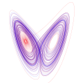  A solution in the Lorenz attractor rendered as an SVG.
• An animation showing trajectories of multiple solutions in a Lorenz system.
• 
  A solution in the Lorenz attractor rendered as a metal wire to show direction and 3D structure.
• An animation showing the divergence of nearby solutions to the Lorenz system.
• 
  A visualization of the Lorenz attractor near an intermittent cycle.
• 
  Two streamlines in a Lorenz system, from ρ = 0 to ρ = 28 (σ = 10, β = ⁠8/3⁠).
• 
  Animation of a Lorenz System with rho-dependence.
• 
  Animation of the Lorenz attractor in the Brain Dynamics Toolbox.^[31]

See also

• Eden's conjecture on the Lyapunov dimension
• Lorenz 96 model
• List of chaotic maps
• Takens' theorem