Slope field

A slope field (also called a direction field^[1]) is a graphical representation of the solutions to a first-order differential equation^[2] of a scalar function. Solutions to a slope field are functions drawn as solid curves. A slope field shows the slope of a differential equation at certain vertical and horizontal intervals on the x-y plane, and can be used to determine the approximate tangent slope at a point on a curve, where the curve is some solution to the differential equation.

The slope field of ${\displaystyle {\frac {dy}{dx}}=x^{2}-x-2}$, with the blue, red, and turquoise lines being ${\displaystyle {\frac {x^{3}}{3}}-{\frac {x^{2}}{2}}-2x+4}$, ${\displaystyle {\frac {x^{3}}{3}}-{\frac {x^{2}}{2}}-2x}$, and ${\displaystyle {\frac {x^{3}}{3}}-{\frac {x^{2}}{2}}-2x-4}$, respectively.

Definition

Standard case

The slope field can be defined for the following type of differential equations

${\displaystyle y'=f(x,y),}$

which can be interpreted geometrically as giving the slope of the tangent to the graph of the differential equation's solution (integral curve) at each point (x, y) as a function of the point coordinates.^[3]

It can be viewed as a creative way to plot a real-valued function of two real variables ${\displaystyle f(x,y)}$ as a planar picture. Specifically, for a given pair ${\displaystyle x,y}$, a vector with the components ${\displaystyle [1,f(x,y)]}$ is drawn at the point ${\displaystyle x,y}$ on the ${\displaystyle x,y}$-plane. Sometimes, the vector ${\displaystyle [1,f(x,y)]}$ is normalized to make the plot better looking for a human eye. A set of pairs ${\displaystyle x,y}$ making a rectangular grid is typically used for the drawing.

An isocline (a series of lines with the same slope) is often used to supplement the slope field. In an equation of the form ${\displaystyle y'=f(x,y)}$, the isocline is a line in the ${\displaystyle x,y}$-plane obtained by setting ${\displaystyle f(x,y)}$ equal to a constant.

General case of a system of differential equations

Given a system of differential equations,

${\displaystyle {\begin{aligned}{\frac {dx_{1}}{dt}}&=f_{1}(t,x_{1},x_{2},\ldots ,x_{n})\\{\frac {dx_{2}}{dt}}&=f_{2}(t,x_{1},x_{2},\ldots ,x_{n})\\&\;\;\vdots \\{\frac {dx_{n}}{dt}}&=f_{n}(t,x_{1},x_{2},\ldots ,x_{n})\end{aligned}}}$

the slope field is an array of slope marks in the phase space (in any number of dimensions depending on the number of relevant variables; for example, two in the case of a first-order linear ODE, as seen to the right). Each slope mark is centered at a point ${\displaystyle (t,x_{1},x_{2},\ldots ,x_{n})}$ and is parallel to the vector

${\displaystyle {\begin{pmatrix}1\\f_{1}(t,x_{1},x_{2},\ldots ,x_{n})\\f_{2}(t,x_{1},x_{2},\ldots ,x_{n})\\\vdots \\f_{n}(t,x_{1},x_{2},\ldots ,x_{n})\end{pmatrix}}.}$

The number, position, and length of the slope marks can be arbitrary. The positions are usually chosen such that the points ${\displaystyle (t,x_{1},x_{2},\ldots ,x_{n})}$ make a uniform grid. The standard case, described above, represents ${\displaystyle n=1}$. The general case of the slope field for systems of differential equations is not easy to visualize for ${\displaystyle n>2}$.

General application

With computers, complicated slope fields can be quickly made without tedium, and so an only recently practical application is to use them merely to get the feel for what a solution should be before an explicit general solution is sought. Of course, computers can also just solve for one, if it exists.

If there is no explicit general solution, computers can use slope fields (even if they aren’t shown) to numerically find graphical solutions. Examples of such routines are Euler's method, or better, the Runge–Kutta methods.

Software for plotting slope fields

Different software packages can plot slope fields.

Direction field code in GNU Octave/MATLAB

funn = @(x, y)y-x;                             % function f(x, y) = y-x
[x, y] = meshgrid(-5:0.5:5);                   % intervals for x and y
slopes = funn(x, y);                           % matrix of slope values
dy = slopes ./ sqrt(1 + slopes.^2);            % normalize the line element...
dx = ones(length(dy)) ./ sqrt(1 + slopes.^2);  % ...magnitudes for dy and dx
h = quiver(x, y, dx, dy, 0.5);                 % plot the direction field
set(h, "maxheadsize", 0.1);                    % alter head size

Example code for Maxima

/* field for y'=xy (click on a point to get an integral curve). Plotdf requires Xmaxima  */
plotdf( x*y, [x,-2,2], [y,-2,2]);

Example code for Mathematica

(* field for y'=xy *)
VectorPlot[{1,x*y},{x,-2,2},{y,-2,2}]

Example code for SageMath^[4]

var('x,y')
plot_slope_field(x*y, (x,0,-5), (y,-5,5))

Examples

• y' = x/y
• 
  Slope field
• 
  Integral curves
• 
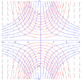  Isoclines (blue), slope field (black), and some solution curves (red)

See also

• Examples of differential equations
• Vector field
• Laplace transform applied to differential equations
• List of dynamical systems and differential equations topics
• Qualitative theory of differential equations